Sometimes, in real-life office situations, or while taking part in a spreadsheet-based test, we have to make predictions based on existing figures and assumptions. Today, we’re going to learn something similar. In this tutorial, we will learn how to predict the number of customers a business will have in 10 years, based on some set assumptions.
Required Tools
The tutorial is specifically made for any version of Microsoft Excel. The same steps should work with Google Sheets with some minor changes.
Formulas / Functions Used
This tutorial uses basic Division, Multiplication, Addition and Subtraction formulas. Absolute Referencing and Decrease Decimal features are also used in this tutorial.
Predicting the Number of Customers a Business will have in 10 Years
Let’s assume that the problem that we’re working with is as below:
XYZ is a software company that currently has 100 customers. Every year, 15% of the customers leave XYZ, and the company acquires 20 new customers. What is the number of customers that XYZ will be having in 10 years?
Step 1: Create an Input Table
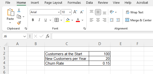
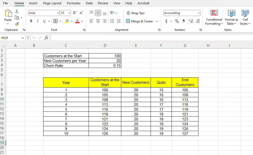
Firstly, let us create an input table and put the information that we already know. The three inputs would be:
- Customers at the Start, which is 100
- New Customers per Year, which is 20
- Churn Rate, which is 0.15
Step 2: Create an Output Table
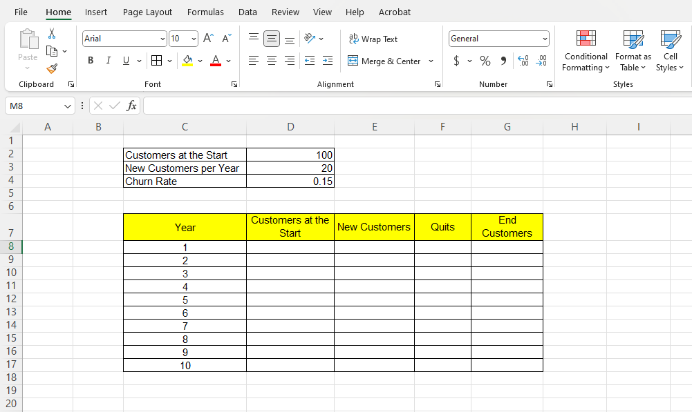
At cell C7, let us create a table with 04 columns, for Year, Customers at the Start, New Customers, Quits, and End Customers. The table should have 11 rows, one for the header and one each for the 10 years.
Step 3: Use Relative Cell Reference to Complete the Table
Now we will use cell reference to fill up the table. The reason we will be doing this instead of putting absolute numbers is so that we can change the inputs if needed, and the outputs will change accordingly. We are going to use the cell references as below:
- At cell D8, we’re going to use the reference =D2
- At cell E8, we’re going to put =$D$3
- At cell F8, we’re going to put =D8*$D$4
- At cell G8, we’re going to put =D8+E8-F8
- At cell D9, we’re going to put =G8
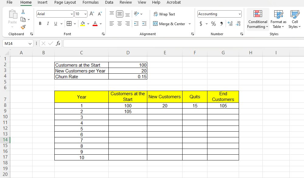
Now, we will select cell D9, and copy the formula to the range D10:D17. Then we will select the range E8:G8, put the cursor at the right bottom corner of the cell G8, and when the cursor changes to a crosshair, we will drag it down to G17.
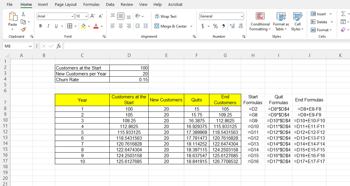
(The function FORMULATEXT has been used in the range H8:J17 to show the formula used in the output table)
Step 4: Use ‘Decrease Decimal’ Feature to Round Up the Numbers
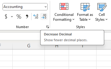
As we can see the numbers are in decimals, where the numbers of customers should be whole numbers. To round up, we select the output table and will click on the ‘Decrease Decimal’ feature from the top ribbon as many times as we need for our table to have only whole numbers.
Now, we should see that the prediction of customers for the next 10 years should appear in the corresponding cells in whole numbers.
Learn More
Here are some similar tutorials that you may find interest in:
- How to calculate how much a business owes its suppliers
- How to calculate profit from sales using spreadsheets
- How to determine the price of a product to ensure profit maximization
- How to calculate the grades of a student from the marks that they obtained
Conclusion
So here’s how to predict the number of customers a business will have in 10 years. If you have any queries regarding this or anything related to spreadsheets, feel free to let us know in the comments or through the Contact page.


