IF function is one of the most popular functions in Excel. It allows you to be a bit creative in the sense that you can command ‘if X happens, then return Y, or else return Z’, and you get to decide what X, Y, and Z would be. In this article, you will learn how to use the IF function in Excel.

Required Tools

The tutorial is specifically made for any version of Microsoft Excel. The same steps should work with Google Sheets with some minor changes.

IF Function in Excel

Syntax

=IF(logical_test, value_if_true, value_if_false)

logical_test: The condition you want to test. It can be an argument or an equation. 

value_if_true: The value that you want Excel to return if the logical_test is true.

value_if_false: The value that you want Excel to return if the logical_test is false.

This means,

• =IF(A1>0,”Yes”,”No”) returns ‘Yes’ if the value in cell A1 is greater than 0, or else, returns ‘No’.
• =IF(A1+B1=C1,”Yes”,””) returns ‘Yes’ if the sum of the values in cells A1 and B1 is equal to the value in cell C1, or else, returns a blank cell (denoted by “”).
• =IF(A1=”Import Range”,”Yes”,”No”) returns ‘Yes’ if the value in cell A1 is the text ‘Import Range’, or else, returns ‘No”.

For example,

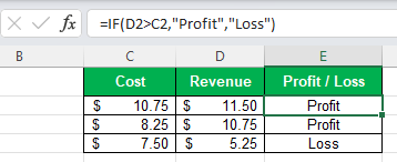
Here at cell E2, the formula =IF(D2>C2,”Profit”,”Loss”) returns ‘Profit’ if the revenue is greater than the cost, and returns ‘Loss’ otherwise (when the cost is equal or greater than the revenue).

Practice

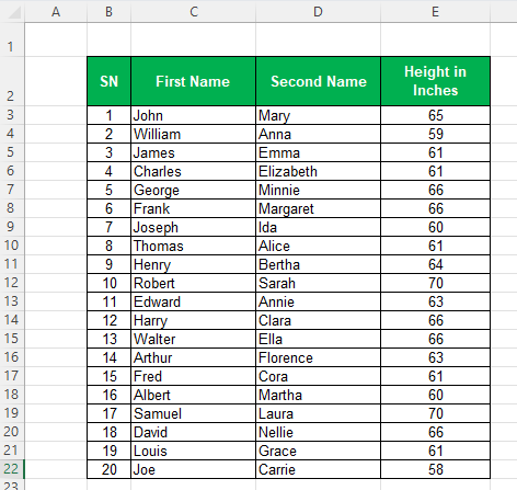
Let’s say we have a dataset for 20 college students where we have their names and heights. We are to select students for a sport in the 65-Inch category. So we have to identify students who have heights equal to or less than 65 inches. It’s also possible to do this with VLOOKUP, filtering with criteria, etc., but here we’re going to do this using the IF function. 

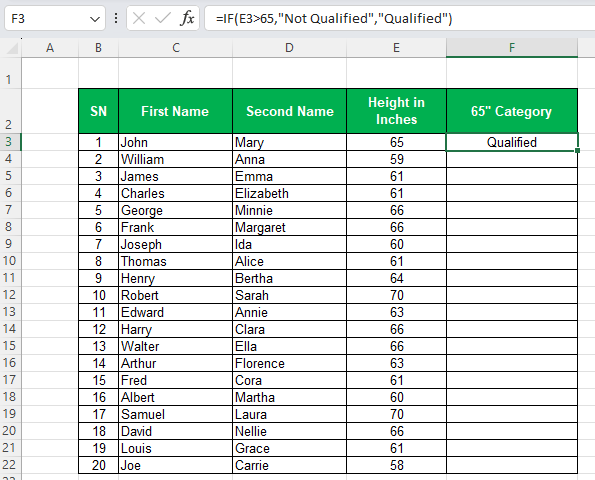
Firstly, we will add a new column F, and at F3, we will use the formula =IF(E3>65,”Not Qualified”,”Qualified”), which means, it will return ‘Not Qualified’, if the value in E3 is greater than 65, or else, it will return ‘Qualified’. Once done, F3 should return ‘Qualified’ as the height of the first student is 65 inches, which is within the range. 

Now, we will have to copy the formula for the range F4:F22. We can do this using any of the following approaches:

• Select the cell F3, and after pressing Ctrl+C, select the range F4:F22 and press Ctrl+V
• Select the cell F3, and after pressing Ctrl+C, select the range F3:F22 and press the Enter key
• Select the cell F3, and after the ‘cross hair’ icon appears at the corner of the cell, drag the formula up to F22

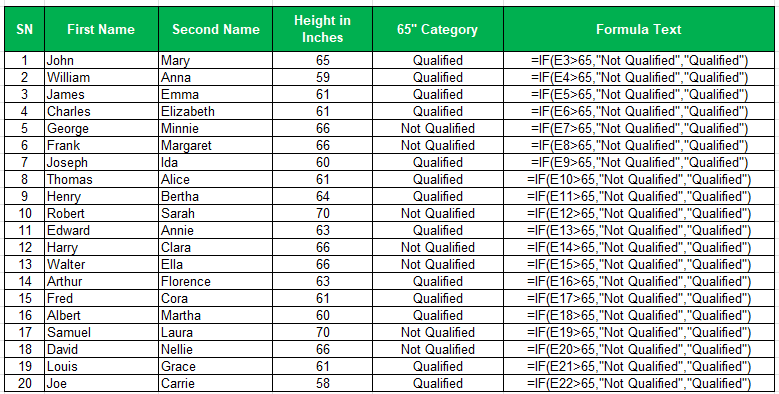
The table should now be completed and column F should identify the students who are qualified for the sport.

(FORMULATEXT function has been used in column G to show the formulas used in column F.)

Download the Practice File

Learn More

Here are some similar tutorials that you might find interest in:

• Excel SUM Function
• Excel VLOOKUP Function
• Excel DATE Function
• Excel INDEX Function

Conclusion

So here’s how to use the Excel IF Function. If you have any queries regarding this or anything related to spreadsheets, feel free to let us know in the comments or through the Contact page.