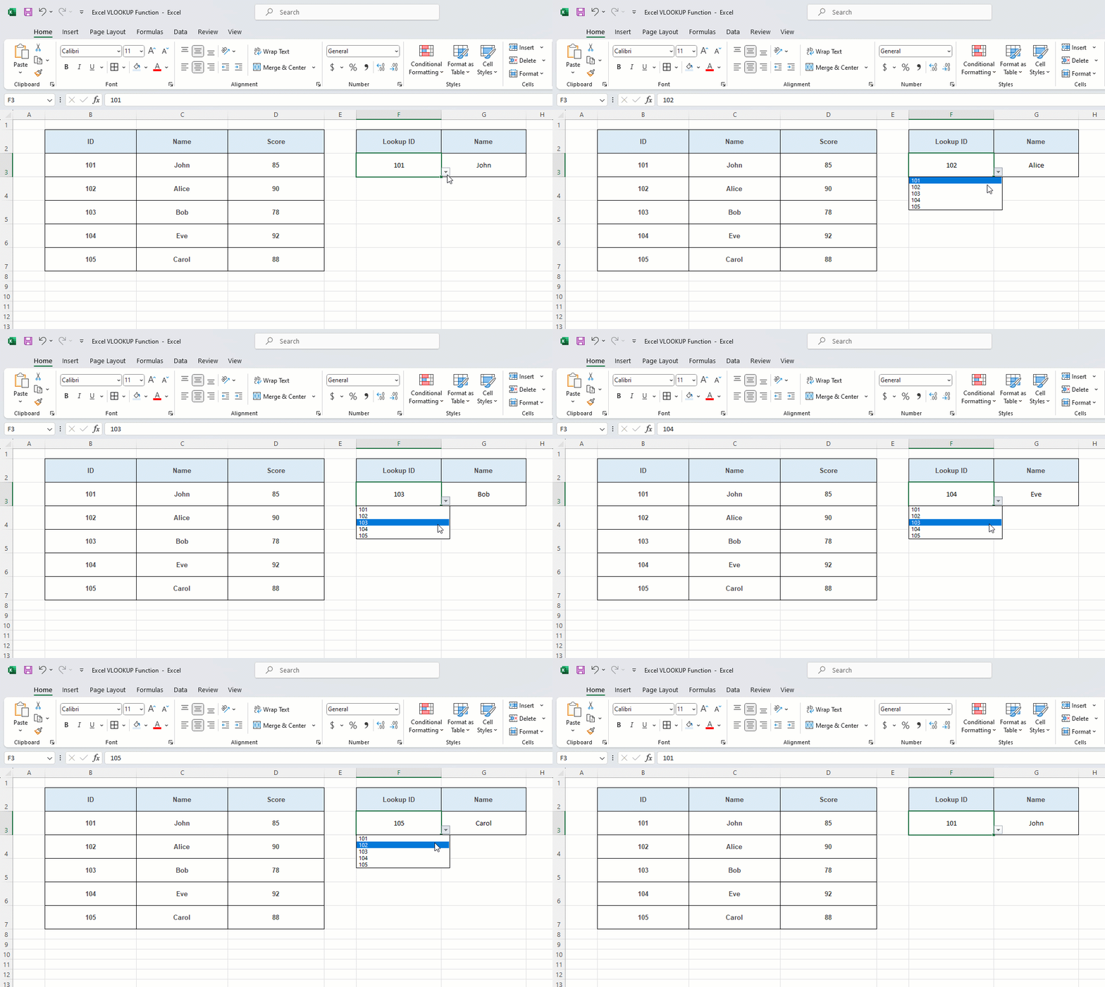
The VLOOKUP function is one of the most commonly used functions in Excel for searching and retrieving data from a specific column in a table. In this article, you will learn how to use the VLOOKUP function to look up and retrieve data efficiently.
Required Tools
The tutorial is specifically made for any version of Microsoft Excel. The same steps should work with Google Sheets with some minor changes.
Excel VLOOKUP Function
Syntax
=VLOOKUP(lookup_value, table_array, col_index_num, range_lookup)
- lookup_value: The value you want to look for in the first column of the table.
- table_array: The range of cells that contains the data. It includes both the column with the lookup value and the column with the value to return.
- col_index_num: The column number in the table from which to retrieve the value.
- range_lookup: [Optional] TRUE for an approximate match or FALSE for an exact match. The default is TRUE.
For example,
=VLOOKUP(“John”, A2:D10, 3, FALSE)
This formula looks for “John” in the first column of the range A2:D10 and returns the value in the third column of the range where “John” is found.
Practice
Let’s say we have a student database with student names, IDs, and scores. We want to find the score of a specific student using their ID.

In F2:G3, we have a lookup table, and whenever there is a student ID in cell F3, we want the corresponding student name in cell G3. To do that, we need to follow these steps:
- Select the Cell: Select the cell where you want the result to appear. For us, it’s cell G3.
- Enter the Formula: Type =VLOOKUP() in the formula bar.
- Specify Lookup Value: Enter the value you want to search for. This can be a direct value or a cell reference. For our case, it’s cell F3.
- Define Table Array: Select the range of cells containing your data. For this example, the range should be B3:C7.
- Column Index Number: Specify the column number in the table from which to retrieve the data. Our expected data (the student name) lies in the second column, hence 2.
- Range Lookup: Enter TRUE (or 1) for an approximate match or FALSE (or 0) for an exact match. We would put FALSE or 0.
So the formula that we will put in cell G3 will be:
=VLOOKUP(F3,B3:C7,2,0)
Now, if there is a value in cell F3, let’s say 103, we will see the cell G3 returning the corresponding name, which is Bob.

We can also use a dropdown list using the ‘Data Validation’ feature under the ‘Data’ tab in cell 3, so that the user can change the ID’s of the student and the corresponding name will change accordingly.

Common Errors and Solutions
- #N/A Error: This error occurs when the lookup value is not found in the first column of the table array. Ensure the lookup value exists and is correctly entered.
- #REF! Error: This occurs if the col_index_num is greater than the number of columns in the table array. Verify the column number.
- #VALUE! Error: This happens if the col_index_num is not a numeric value. Make sure to enter a valid number.
Tips and Best Practices
- Use Absolute References: When copying the VLOOKUP formula to multiple cells, use absolute references for the table array to keep it consistent.
- Ensure Sorted Data for Approximate Match: If using TRUE for range_lookup, ensure the first column of the table array is sorted in ascending order.
- Use Named Ranges: For easier readability and maintenance, use named ranges for the table array.
Learn More
Here are some similar tutorials that you might find interest in:
Conclusion
The VLOOKUP function is a powerful tool in Excel for retrieving data based on specific criteria. By understanding its syntax and usage, you can enhance your data analysis skills significantly. If you have any queries regarding this or anything related to spreadsheets, feel free to let us know in the comments or through the Contact page.


