One of the very common uses of spreadsheets is creating grades for students. Chances are that the grade sheets that we received in our schools (or that you receive if you’re currently a student) are all made using spreadsheets. In this tutorial, we will learn how to calculate the grades of a student using spreadsheets.
Required Tools
The tutorial is specifically made for any version of Microsoft Excel. The same steps should work with Google Sheets with some minor changes.
Formulas / Functions Used
This tutorial uses VLOOKUP function to determine the grading of the student. Absolute Referencing is used here as well.
Calculating the Grades of a Student using Spreadsheets
For this example, we’re going to follow the following criteria for the grading:
- 0-59 would be equivalent to F
- 60-69 would be equivalent to B
- 70-79 would be equivalent to B+
- 80-89 would be equivalent to A
- 90-100 would be equivalent to A+
Step 1: Create the Criteria for the Grading
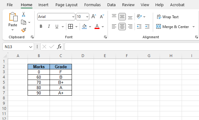
Let’s put the first numbers of the ranges in a table along with the equivalent grades. For instance, while our range for B is 60-69, we will put only 60 for B, 70 for B+ and so on.

Step 2: Create the Mark Sheet
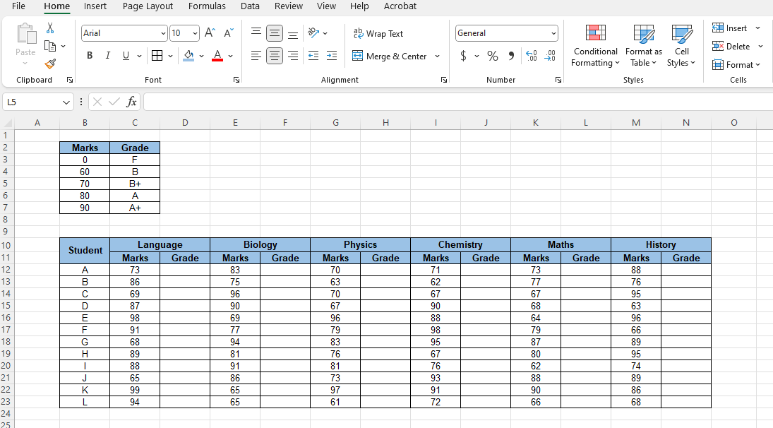
Let’s assume we have the marks of 12 students for 6 subjects. We have used random numbers between 60 and 100 for this example. Let’s put the marks in a table in such a way that there are two columns for each subject, one for the marks, and the other for the grades.

Step 3: Use the VLOOKUP Function to Calculate the Grades
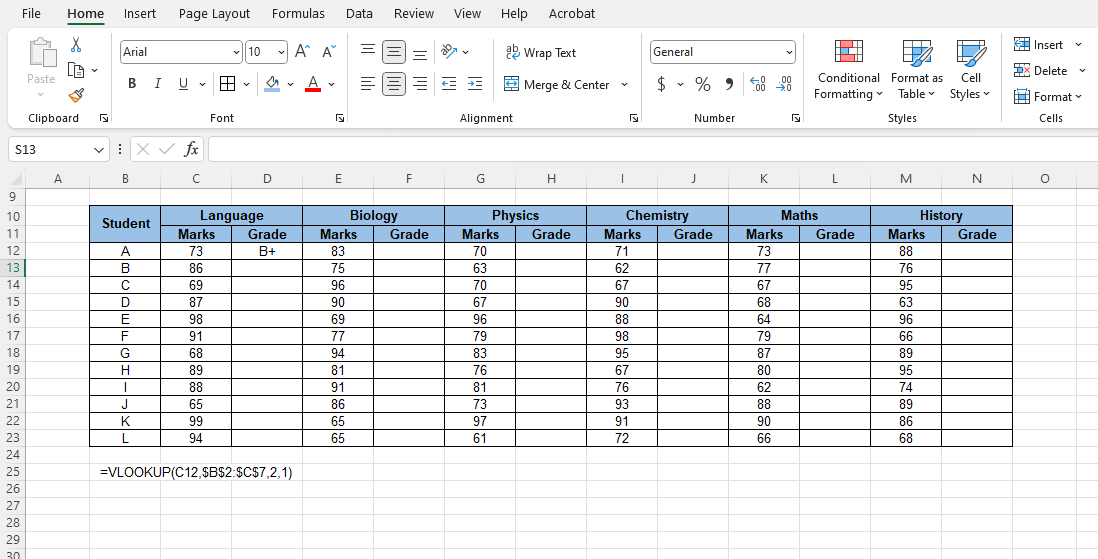
At cell D12, let’s use the formula, =VLOOKUP(C12,$B$2:$C$7,2,1) to determine the grade of Student A for Language, and we will see that the equivalent grade (B+) appears in the cell. Absolute reference has been used for the range B2:C7 as we want the criteria to be always pulled from this specific range. Also, we have used the approximate match for VLOOKUP instead of the exact match, as we want excel to determine the grades from a set of ranges and not from a set of exact numbers.

(The FORMULATEXT function has been used in cell C25 to show the formula used in cell D12)
Step 4: Copy the Formula to Complete the Table
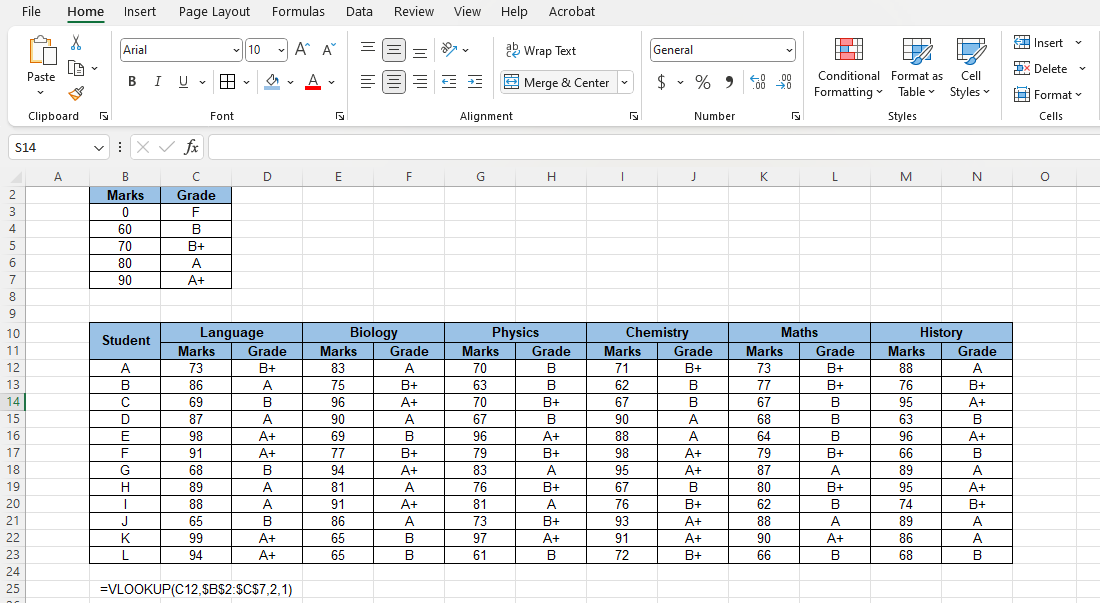
Let’s put the cursor in the right bottom corner of cell D12, and drag down the crosshair to copy the formula to the range D13:D23. We can see that the grades for Language for all the students have appeared. Now, let us select the range D12:D23, copy using Ctrl +C, click on cell F12, and paste using Ctrl + V. The grades for Biology for all the students should appear as well. In the same way, we will paste the formula from the range D12:D23 to H12, J12, L12, and N12 respectively to complete the table.

Learn More
Here are some similar tutorials that you may find interest in:
- How to calculate how much a business owes its suppliers
- How to calculate profit from sales using spreadsheets
- How to determine the price of a product to ensure profit maximization
- How to predict the number of customers a Business will have in 10 Years
Conclusion
So here’s how to calculate the grades of a student using spreadsheets. If you have any queries regarding this or anything related to spreadsheets, feel free to let us know in the comments or through the Contact page.


