Pricing is one of the key tools for any marketing strategy. It’s important to set the right price as changing prices has a direct impact on demand and sales. In this tutorial, we will learn how to determine the price of a product to ensure profit maximization, and we will do it using spreadsheets.
Required Tools
The tutorial is specifically made for any version of Microsoft Excel. The same steps should work with Google Sheets with some minor changes.
Formulas / Functions Used
This tutorial uses basic Division, Multiplication, Addition and Subtraction formulas. Absolute Referencing is used here as well. For a larger dataset, Conditional Formatting may be further useful, which is explained in the tutorial.
Determining the Price of a Product to Ensure Profit Maximization
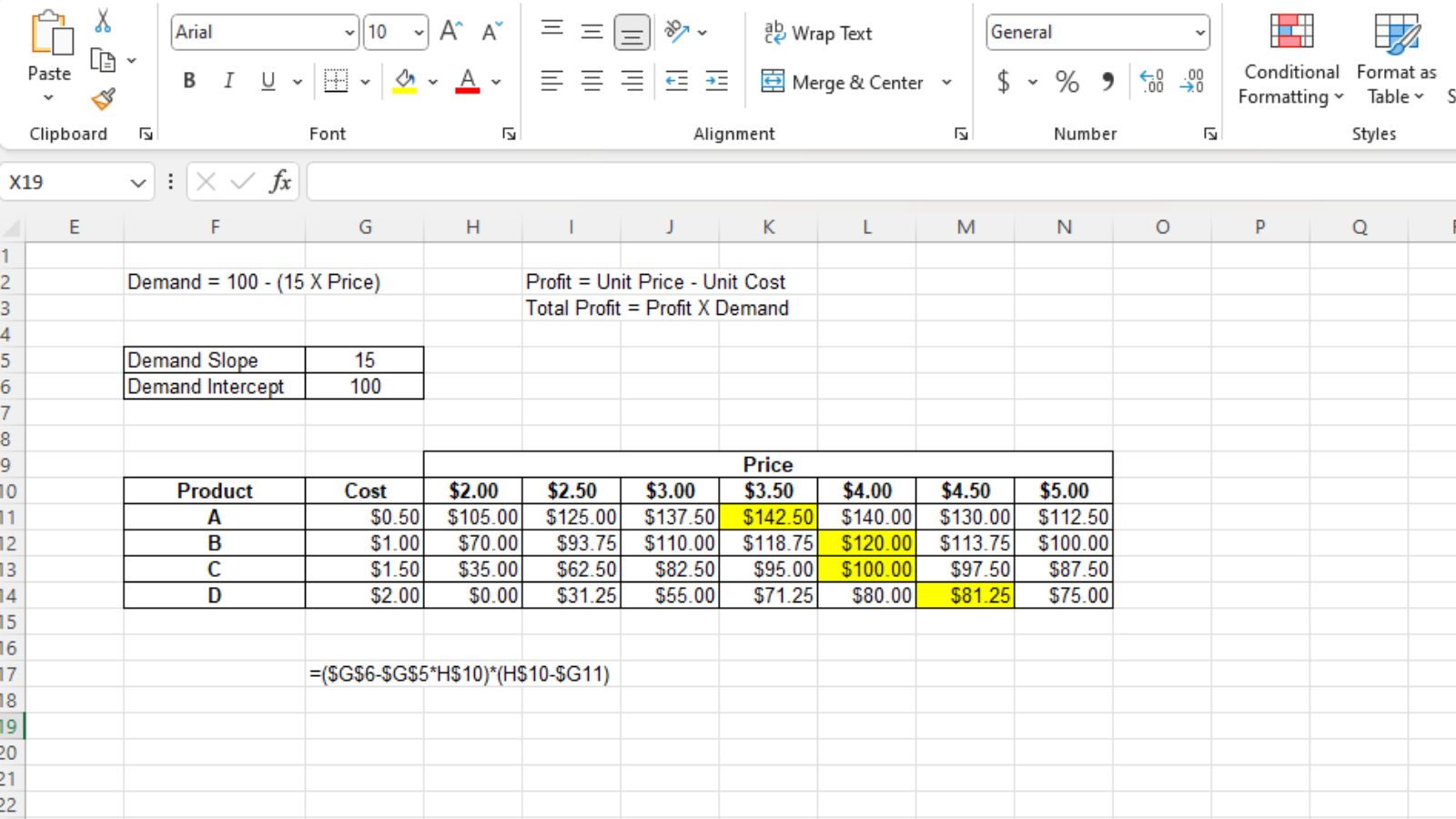
We know that Profit Margin = Unit Price – Unit Cost, and Total Profit = Profit x Demand. Let’s assume that our Demand Slope is 15 and the Demand Intercept is 100. That means, Demand = 100 – (15 x Price). We have 04 products that cost as below:
- Product A costs $0.50
- Product B costs $1.00
- Product C costs $1.50
- Product D costs $2.00
We have to identify the best price for each of these products, while the prices must be within the range of $2.00 – $5.00.
Step 1: Create an Input Table
Let’s create an input table with two variables that are Demand Slope and Demand Intercept. This is so that we can change these two figures if we want. According to the situation, the slope is 15 and the intercept is 100.
Step 2: Create an Output Table with Costs and Prices
At cell F10, let’s create a table, put the costs of each product vertically, and put the potential prices for each product horizontally.
Step 3: Calculate the Total Profit at Each Price
As we can understand, the formula for total profit at each price would be:
Demand x Profit
= (Intercept – Slope x Price) x (Unit Price – Unit Cost)
So at H11, we will use the formula =($G$6-$G$5*H$10)*(H$10-$G11) and the profit for product A at $2.00 should appear there.
Absolute reference (dollar sign) is used for G5 and G6 because we do not want the row or column to change as we copy our formulas. We have locked the row of cell H10 for the formula as the price will always be pulled from row 10. We have also locked the column of cell G11 for the formula as the cost will always be pulled from column G.
(The FORMULATEXT function has been used in cell G17 to show the formula used in cell H11)
Step 4: Identify the Price with Maximum Profit for Each Product
For each of the products, we have to identify the prices that maximize the total profit. For example, for product A, we find the largest number from the range H11:N11. The largest number happens to be $142.50 at cell K11, so the corresponding price at K10 ($3.50) is the best price for product A. In the same way, we can see that $4.00 will be the best price for products B and C, while $4.50 is the best price for product D.
We can use an Excel feature to find and highlight the maximum number from a range which is Conditional Formatting, which can be particularly useful for a larger dataset.
Download the Practice FileLearn More
Here are some similar tutorials that you may find interest in:
- How to calculate how much a business owes its suppliers
- How to calculate profit from sales using spreadsheets
- How to predict the number of customers a business will have in 10 Years
- How to calculate the grades of a student from the marks that they obtained
Conclusion
So here’s how to determine the price of a product to ensure profit maximization. If you have any queries regarding this or anything related to spreadsheets, feel free to let us know in the comments or through the Contact page.


